Approximating continuously defined functions from given discrete data is an unavoidable task in various fields. Interpolation represents the relatively easiest approach, where an approximating function is constructed that has to perfectly agree with the given points.
If x_0 \ldots x_n and f(x_0) \ldots f(x_n) are known and if x_0 < x < x_n, then the estimated value of f(x) is said to be an Interpolation. If x < x_0 or x > x_n then the estimated value is said to be an Extrapolation.
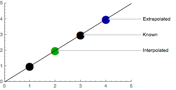
In other words: with interpolation, we want to estimate values between already known values, and with extrapolation, we want to estimate values outside already known values.
Polynomial Interpolation
Polynomial interpolation interpolates a given data set by the polynomial of the lowest possible degree that passes through all the dataset points. Interpolation inevitably leads to a problem in linear algebra where we have to solve a system of linear equations.
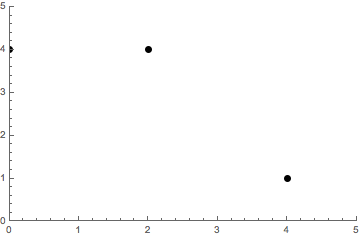
Let’s work through an example with the points
(0, 4)\qquad (2, 4)\qquad (4, 1).
The example points can be visualized as follows.
Direct Interpolation
We need at least n + 1 data points to solve a polynomial of degree n.
The resulting polynomial is unique because an n-degree polynomial has at most n roots.
Suppose we interpolate through n + 1 data points with a polynomial p(x) of degree \leq n. Suppose another polynomial q(x) exists also of degree \leq n that also interpolates the n + 1 points.
- Consider r(x) = p(x) - q(x)
We know that r(x) is is a polynomial of degree at most n because we are just subtracting polynomials. At the n + 1 data points r(x_i) = p(x_i) -q(x_i) = 0, therefore r(x) has n + 1 roots.
- We get r(x) = 0
By the fundamental theorem of algebra r(x) can only have more than n roots if r(x) = 0.
- Therefore r(x) = 0 \implies p(x) = q(x)
The direct method assumes the following polynomial:
y=f(x)=c_0+c_1x + c_2 x^2 + \ldots + c_n x^n
With n + 1 given points (x_0,y_0) \ldots (x_n,y_n) we have to solve n + 1 linear equations to find all coefficients c_0, c_1,\ldots, c_n for the interpolating polynomial of degree n.
\begin{aligned} 4 = c_0 + 0c_1 + 0^2c_2 \\ 4 = c_0 + 2c_1 + 2^2c_2 \\ 1 = c_0 + 4c_1 + 4^2c_2 \end{aligned}
This linear system of equations can be described by a special kind of matrix known as the Vandermonde Matrix.
\left( \begin{array}{ccc} 1 & 0 & 0 \\ 1 & 2 & 4 \\ 1 & 4 & 16 \\ \end{array} \right) \left( \begin{array}{ccc} c_0 \\ c_1 \\ c_2 \\ \end{array} \right) = \left( \begin{array}{ccc} 4 \\ 4 \\ 1 \\ \end{array} \right)
The polynomial basis looks like B = \{1, x, x^2, \ldots, x^n\}, as represented by the columns of the Vandermonde matrix. Our resulting interpolating polynomial is a linear combination of this basis.
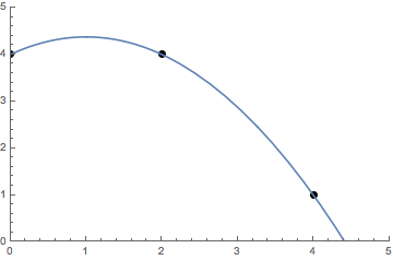
P(x) = 4 + \frac{3}{4}x - \frac{3}{8}x^2
Unfortunately, we have to invert the Vandermonde matrix to solve for the coefficients c_0, c_1 \ldots, c_n. Let’s see if we can find a better basis to find the coefficients.
Lagrange Interpolation
Lagrange polynomials are based on the beautiful idea that you could express the interpolating polynomial P as a linear combination of polynomials p_0 \ldots p_n, that individually fit a specific given point.1
We will arrive at the same unique polynomial that we have calculated before but with a completely different way of constructing it.
Our goal is to create multiple polynomials that are 1 at a specific point (x_i, y_i) and 0 at all other given points.
Let’s create a polynomial p(x) = (x - 0)(x - 2)(x - 4) that is 0 at all values for x. We will now create polynomials that individually cancel out one of the terms.
\begin{aligned} p_0(x) = p(x)/(x - 0) \\ p_1(x) = p(x)/(x - 2) \\ p_2(x) = p(x)/(x - 4) \end{aligned}
Each of these polynomials is 1 at a point x_i, and simultaneously 0 at all other points. Because we know the values y_i for each x_i, we have found our coefficients without having to invert a matrix!
Notice that we can now create a basis B = \{\frac{p_0(x)}{p_0(x_0)}, \frac{p_1(x)}{p_1(x_1)}, \ldots, \frac{p_n(x)}{p_n(x_n)}\} for which we know that the coefficients are y_0, y_1 \ldots y_n. We can again write the polynomial P as a linear combination of our new basis B.
P(x) = 4 \frac{p_0(x)}{p_0(0)} + 4 \frac{p_1(x)}{p_1(2)} + 1 \frac{p_2(x)}{p_2(4)}
Keep in mind that this intuitive way of writing Lagrange polynomials requires simplification before evaluation to avoid division by zero.
P(x) = 4 + \frac{3}{4}x - \frac{3}{8}x^2
Newton Interpolation
One of the most important features of Newton’s interpolation method is that we can gradually increase the interpolated data points without recomputing what is already computed.
When an additional point (x_{n+1}, y_{n+1}) is to be used, all previous basis polynomials and their corresponding coefficients remain unchanged, and we only need to obtain a new basis polynomial of degree n + 1.
Let’s calculate the Newton interpolation for our example.2
\begin{aligned} 4 = c_0 + c_1(0 - 0) + c_2(0 - 0)(0 - 2) \\ 4 = c_0 + c_1(2 - 0) + c_2(2 - 0)(2 - 2) \\ 1 = c_0 + c_1(4 - 0) + c_2(4 - 0)(4 - 2) \\ \end{aligned}
We can simplify that expression and write it in matrix form
\left( \begin{array}{ccc} 1 & 0 & 0 \\ 1 & 2 - 0 & 0 \\ 1 & 4 - 0 & (4 - 0)(4 - 2) \\ \end{array} \right) \left( \begin{array}{ccc} c_0 \\ c_1 \\ c_2 \\ \end{array} \right) = \left( \begin{array}{ccc} 4 \\ 4 \\ 1 \\ \end{array} \right).
We can solve that system of linear equations progressively from top to bottom without having to invert the matrix. In contrast to the other interpolation methods, the basis now looks like
B = \{1, (x - x_0), (x - x_0)(x - x_1), \ldots, \prod_{i=0}^n(x - x_i)\}.
If we need to interpolate another point, we can reuse our previous results and solve another row.
P(x) = 4 + 0(x-0) - \frac{3}{8}(x-0)(x-2) = 4 + \frac{3}{4}x - \frac{3}{8}x^2
Runge’s Phenomenon
We have now seen that all polynomial interpolation methods for n + 1 data points result in the same unique polynomial of degree n. All of the methods for polynomial interpolation were expressed in terms of a basis B weighted by some coefficients. The interpolating polynomial for our previous example looks as follows.
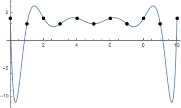
A problem that arises with polynomial interpolation is the interpolating function tends to oscillate more and more with more points added. This is called the Runge’s phenomenon. It limits the use cases where simple polynomial interpolation is appropriate.
Another limitation of polynomial interpolation is that touching a single point causes a recalculation of all other points.
Piecewise Interpolation
To address the limitations mentioned, we could combine multiple polynomials of lower degree that each fit an interval between two points.
S(x)= \left\{\begin{array}{cc} P_0(x) & x_0 \le x \le x_1 \\ \vdots & \vdots\\ P_n(x) & x_{n-1} \le x \le x_n \end{array}\right.
The function S(x) defined by piecewise polynomials is known as a Spline. We usually want a spline interpolation to consist of low-degree polynomials, to be continuous and to be smooth.
In other words we want two consecutive piecewise polynomials to meet at some point P_i(x_i) = P_{i + 1}(x_i) and to have the same derivative at that point P_i^{(k)}(x_i) = P_{i + 1}^{(k)}(x_i) where k stands for the kth-derivative.
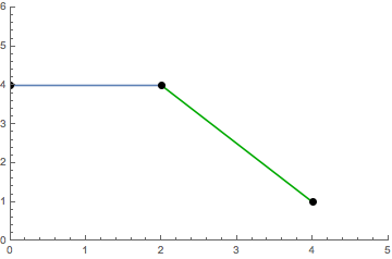
Linear Splines
A linear spline, as the name implies, describes first-degree polynomials of the form P(x) = c_0 + c_1 x. Each linear polynomial has 2 unkown parameters, our spline of n piecewise polynomials for n + 1 data points thus has a total of 2n unknown parameters.
The continuity condition, that consecutive polynomials to meet at some point, needs 2n free parameters to be fulfilled. Linear splines can thus only fulfill that condition.
\begin{aligned} P_0x_{i - 1}) &= a_0 + a_1 x_{i - 1} & 4 &= a_0 + 0 a_1 \\ P_0(x_i) &= a_0 + a_1 x_i & 4 &= a_0 + 2 a_1 \\ P_1(x_i) &= b_0 + b_1 x_i & 4 &= b_0 + 2 b_1 \\ P_1(x_{i + 1}) &= b_0 + b_1 x_{i + 1} & 1 &= b_0 + 4 b_1 \end{aligned}
This leads to a major drawback of linear splines: they are not smooth and hence are usually not differentiable at points where two consecutive polynomials meet.
S(x)= \left\{\begin{array}{lc} P_0(x) = 4 & 0 \le x \le 2 \\ & \\ P_1(x) = 7 - \frac{3}{2}x & 2 \le x \le 4 \end{array}\right.
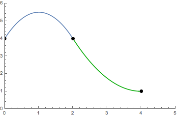
Quadratic Splines
Quadratic polynomials add one more degree of freedom, and quadratic splines consequently have 3n unknown parameters. Again, we need 2n parameters for continuity, but we can now also specify that two consecutive polynomials should match in their first derivative.
The smoothness condition needs n - 1 free parameters, because there are n - 1 “inner points” for n + 1 data points.
\begin{aligned} P_0(x_{i - 1}) &= a_0 + a_1 x_{i - 1} + a_2 x_{i - 1}^2 & 4 &= a_0 + 0 a_1 + 0^2 a_2 \\ P_0(x_i) &= a_0 + a_1 x_i + a_2 x_i^2 & 4 &= a_0 + 2 a_1 + 2^2 a_2 \\ P_1(x_i) &= b_0 + b_1 x_i + b_2 x_i^2 & 4 &= b_0 + 2 b_1 + 2^2 b_2 \\ P_1(x_{i + 1}) &= b_0 + b_1 x_{i + 1} + b_2 x_{i + 1}^2 & 1 &= b_0 + 4 b_1 + 4^2 b_2 \end{aligned}
We need another equation (n - 1 = 1) to make sure that two consecutive polynomials have a common first derivative.
P_0'(x_i) = P_1'(x_i)\qquad a_1 + 4 a_2 = b_1 + 4 b_2
Now, we have a total of 5 equations for 3n = 6 unknown parameters. For us to be able to solve the equations we have 3n - 2n - (n - 1) = 1 free parameter left. We can choose one more solvable constraint of our liking, for example, that the first derivative should be 0 at the last point.
P_1'(x_n) = 0\qquad 0 = b_1 + 8 b_2
Our quadratic spline is now defined as
S(x)= \left\{\begin{array}{lc} P_0(x) = 4 + 3x - \frac{3}{2}x^2 & 0 \le x \le 2 \\ & \\ P_1(x) = 13 - 6x + \frac{3}{4}x^2 & 2 \le x \le 4 \end{array}\right..
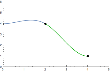
Cubic Splines
With another degree of freedom, we can specify that two consecutive polynomials share a common first and second derivative at the point they meet.
We now have 4n unknown parameters of which 2n are bound by the continuity condition.
\begin{aligned} P_0(x_{i - 1}) &= a_0 + a_1 x_{i - 1} + a_2 x_{i - 1}^2 + a_3 x_{i - 1}^3 & 4 &= a_0 + 0 a_1 + 0^2 a_2 + 0^3 a_3 \\ P_0(x_i) &= a_0 + a_1 x_i + a_2 x_i^2 + a_3 x_i^3 & 4 &= a_0 + 2 a_1 + 2^2 a_2 + 2^3 a_3 \\ P_1(x_i) &= b_0 + b_1 x_i + b_2 x_i^2 + b_3 x_i^3 & 4 &= b_0 + 2 b_1 + 2^2 b_2 + 2^3 b_3 \\ P_1(x_{i + 1}) &= b_0 + b_1 x_{i + 1} + b_2 x_{i + 1}^2 + b_3 x_{i + 1}^3 & 1 &= b_0 + 4 b_1 + 4^2 b_2 + 4^3 b_3 \end{aligned}
A further 2(n - 1) parameters are bound by the smoothness condition for the first and second derivatives.
\begin{aligned} P_0'(x_i) &= P_1'(x_i) & a_1 + 4 a_2 + 12 a_3 &= b_1 + 4 b_2 + 12 b_3 \\ P_0''(x_i) &= P_1''(x_i) & 2 a_2 + 12 a_3 &= 2 b_2 + 12 b_3 \end{aligned}
We now have 4n - 2n - 2(n - 1) = 2 parameters left for constraints of our choice, which is often exactly what we want for spline interpolation.
\begin{aligned} P_0''(x_0) &= 0 & a_1 = 0 \\ P_1''(x_n) &= 0 & b_1 + 8 b_2 + 48 b_3 = 0 \end{aligned}
Our cubic spline is now defined as
S(x)= \left\{\begin{array}{lc} P_0(x) = 4 + \frac{9}{16}x^2 - \frac{9}{32}x^3 & 0 \le x \le 2 \\ & \\ P_1(x) = -2 + 9x - \frac{63}{16}x^2 + \frac{15}{32}x^3 & 2 \le x \le 4 \end{array}\right..
The following constraints are often used for the two free parameters:
- Natural cubic splines have their second derivative at the first and last point set to zero. P_0''(x_0) = 0 and P_n''(x_n) = 0.
- Complete cubic splines use the first derivative of the function to be interpolated if known P_0'(x_0) = f'(x_0) and P_n'(x_n) = f'(x_n)
- Correct cubic splines use the second derivative of the function to be interpolated if known P_0''(x_0) = f''(x_0) and P_n''(x_n) = f''(x_n).
Finally, we have covered all the basics about splines!3
MathTheBeautiful offers a series of videos on polynomial interpolation that contains an introduction to Lagrange polynomials.↩︎
Ruye Wang wrote a more in-depth tutorial on Newton interpolation and other interpolation methods, which can be found here.↩︎
For more information about splines, the University of Houston offers a great tutorial on how to calculate different splines.↩︎
Updates and Corrections
The source for this article is available at Github. If you want to suggest a change, please create an issue on GitHub.
Citations and Reuse
Figures, and text are licensed under Creative Commons Attribution CC-BY 4.0, unless noted otherwise. The figures that have been reused from other sources don't fall under this license and can be recognized by a note in their caption.